Tutorial¶

This tutorial will walk you through the creation of your first PySB model. It will cover the basics, provide a guide through the different programming constructs and finally deal with more complex rule-building. Users will be able to write simple programs after finishing this section. In what follows we will assume you are issuing commands from a Python prompt (whether it be actual Python or a shell such as iPython. See Getting Started for details).

Note

Familiarity with rules-based biomodel encoding tools such as BioNetGen or Kappa would be useful to users unfamiliar with Rules-based approaches to modeling. A short About Rules is included for new users.

Note

Although a new user can go through the tutorial to understand how PySB works, a basic understanding of the Python programming language is essential. See the Getting Started section for some Python suggestions.

Modeling with PySB¶

A biological model in PySB will need the following components to generate a mathematical representation of a system:

Model definitions: This instantiates the model object.
Monomer definition: This instantiates the monomers that are allowed in the model.
Parameters: These are the numerical parameters needed to create a mass-action or stochastic simulation.
Rules: These are the set of statements that describe how monomer species, interact as prescribed by the parameters involved in a given rule. The collection of these rules is called the model topology.

The following examples will be taken from work in the Sorger lab in extrinsic apoptosis signaling. The initiator caspases, activated by an upstream signal, play an essential role activating the effector Bcl-2 proteins downstream. In this model, Bid is catalitically truncated and activated by Caspase-8, an initiator caspase. We will build a model that represents this activation as a two-step process as follows:

$C8 + Bid \underset{kr}{\overset{kf}{\leftrightharpoons}} C8:Bid \quad {\longleftarrow \mbox{Complex formation step}} \\ C8:Bid \overset{kc}{\rightarrow} C8 + tBid \quad {\longleftarrow \mbox{Complex dissociation step}}$

Where tBid is the truncated Bid. The parameters kf, kr, and kc represent the forward, reverse, and catalytic rates that dictate the consumption of Bid via catalysis by C8 and the formation of tBid. We will eventually end up with a mathematical representation that will look something like this:

(1) $\frac{d[C8]}{dt} &= -kf[C8]*[Bid] + kr*[C8:Bid] + kc*[C8:Bid] \\ \frac{d[Bid]}{dt} &= -kf*[C8]*[Bid] + kr*[C8:Bid] \\ \frac{d[C8:Bid]}{dt} &= kf*[C8]*[Bid] - kr*[C8:Bid] - kc*[C8:Bid] \\ \frac{dt[tBid]}{dt} &= kc*[C8:Bid]$

The species names in square braces represent concentrations, usually give in molar (M) and time in seconds. These ordinary differential equations (ODEs) will then be integrated numerically to obtain the evolution of the system over time. We will explore how a model could be instantiated, modified, and expanded without having to resort to the tedious, repetitive, and error-prone writing and rewriting of equations as those listed above.

The Empty Model¶

We begin by creating a model, which we will call mymodel. Open your favorite Python code editor and create a file called mymodel.py. The first lines of a PySB program must contain these lines so you can type them or paste them in your editor as shown below. Comments in the Python language are denoted by a hash (#) in the first column.

# import the pysb module and all its methods and functions
from pysb import *

# instantiate a model
Model()

Now we have the simplest possible model – the empty model!

To verify that your model is valid and your PySB installation is working, run mymodel.py through the Python interpreter by typing the following command at your command prompt:

python mymodel.py

If all went well, you should not see any output. This is to be expected, because this PySB script defines a model but does not execute any contents. We will revisit these concepts once we have added some components to our model.

Monomers¶

Chemical species in PySB, whether they are small molecules, proteins, or representations of many molecules are all derived from Monomers. Monomers are the superunit that defines how a species can be defined and used. A Monomer is defined using the keyword Monomer followed by the desired monomer name and the sites relevant to that monomer. In PySB, like in BioNetGen or Kappa, there are two types of sites, namely bond-making/breaking sites and state sites. The former allow for the description of bonds between species while the latter allow for the assignment of states to species. Following the first lines of code entered into your model in the previous section we will add a monomer named ‘Bid’ with a bond site ‘b’ and a state site ‘S’. The state site will contain two states, the untruncated (u) state and the truncated (t) state as shown:

Monomer('Bid', ['b', 'S'], {'S':['u', 't']})

Note that this looks like a Python function call. This is because it is in fact a Python function call! [1] The first argument to the function is a string (ecnlosed in quotation marks) specifying the monomer’s name and the second argument is a list of strings specifying the names of its sites. Note that a monomer does not need to have state sites. There is also a third, optional argument for specifying whether any of the sites are “state sites” and the list of valid states for those sites. We will introduce state sites later.

Let’s define two monomers in our model, corresponding to Caspase-8, an initiator caspase involved in apoptosis (C8) and BH3-interacting domain death agonist (Bid) (ref?):

Monomer('C8', ['b'])
Monomer('Bid', ['b', 'S'])

Note that although the C8 monomer only has one site ‘b’, you must still use the square brackets to indicate a list of binding sites. Anticipating what comes below, the 'S' site will become a state site and hence, we choose to represent it in upper case but this is not mandatory.

Now our model file should look like this:

# import the pysb module and all its methods and functions
from pysb import *

# instantiate a model
Model()

# declare monomers
Monomer('C8', ['b'])
Monomer('Bid', ['b', 'S'], {'S':['u', 't']})

We can run python mymodel.py again and verify there are no errors, but you should still have not output given that we have not done anything with the monomers. Now we can do something with them.

Run the ipython (or python) interpreter with no arguments to enter interactive mode (be sure to do this from the same directory where you’ve saved mymodel.py) and run the following code:

>>> import mymodel as m
>>> m.model.monomers

You should see the following output:

Monomer(name='C8', sites=['b'], site_states={})
Monomer(name='Bid', sites=['b', 'S'], site_states={})

In the first line, we treat mymodel.py as a module [2] and import its symbol model. In the second and third lines, we loop over the monomers attribute of model, printing each element of that list. The output for each monomer is a more verbose, explicit representation of the same call we used to define it. [3]

Here we can start to see how PySB is different from other modeling tools. With other tools, text files are typically created with a certain syntax, then passed through an execution tool to perform a task and produce an output, whether on the screen or to an output file. In PySB on the other hand we write Python code defining our model in a regular Python module, and the elements we define in that module can be inspected and manipulated as Python objects interactively in one of the Python REPLs such as iPython or Python. We will explore this concept in more detail in the next section, but for now we will cover the other types components needed to create a working model.

Parameters¶

A Parameter is a named constant floating point number used as a reaction rate constant, compartment volume or initial (boundary) condition for a species (parameter in BNG). A parameter is defined using the keyword Parameter followed by its name and value. Here is how you would define a parameter named ‘kf1’ with the value $4 \times 10^{-7}$ :

Parameter('kf1', 4.0e-7)

The second argument may be any numeric expression, but best practice is to use a floating-point literal in scientific notation as shown in the example above. For our model we will need three parameters, one each for the forward, reverse, and catalytic reactions in our system. Go to your mymodel.py file and add the lines corresponding to the parameters so that your file looks like this:

# import the pysb module and all its methods and functions
from pysb import *

# instantiate a model
Model()

# declare monomers
Monomer('C8', ['b'])
Monomer('Bid', ['b', 'S'], {'S':['u', 't']})

# input the parameter values
Parameter('kf', 1.0e-07)
Parameter('kr', 1.0e-03)
Parameter('kc', 1.0)

Once this is done start the ipython (or python) intepreter and enter the following commands:

>>> import mymodel as m
>>> m.model.parameters

and you should get an output such as:

{'kf': Parameter(name='kf', value=1.0e-07),
 'kr': Parameter(name='kr', value=1.0e-03),
 'kc': Parameter(name='kc', value=1.0    )}

Your model now has monomers and parameters specified. In the next section we will specify rules, which specify the interaction between species and parameters.

Warning

PySB or the integrators that we suggest for use for numerical manipulation do not keep track of units for the user. As such, the user is responsible for keeping track of the model in units that make sense to the user! For example, the forward rates are typically in $M^{-1}s^{-1}$ , the reverse rates in $s^{-1}$ , and the catalytic rates in $s^{-1}$ . For the present examples we have chosen to work in a volume size of $1.0 pL$ corresponding to the volume of a cell and to specify the Parameters and Initial conditions in numbers of molecules per cell. If you wish to change the units you must change all the parameter values accordingly.

Rules¶

Rules, as described in this section, comprise the basic elements of procedural instructions that encode biochemical interactions. In its simplest form a rule is a chemical reaction that can be made general to a range of monomer states or very specific to only one kind of monomer in one kind of state. We follow the style for writing rules as described in BioNetGen but the style proposed by Kappa is quite similar with only some differences related to the implementation details (e.g. mass-action vs. stochastic simulations, compartments or no compartments, etc). We will write two rules to represent the interaction between the reactants and the products in a two-step manner as described in the About Rules section.

The general pattern for a rule consists of the statement Rule and in parenthesis a series of statements separated by commas, namely the rule name (string), the rule interactions, and the rule parameters. The rule interactions make use of the following operators:

*+* operator to represent complexation
*<>* operator to represent backward/forward reaction
*>>* operator to represent forward-only reaction
*%* operator to represent a binding interaction between two species

To illustrate the use of the operators and the rule syntax we write the complex formation reaction with labels illustrating the parts of the rule:

Rule('C8_Bid_bind', C8(b=None) + Bid(b=None, S='u') <> C8(b=1) % Bid(b=1, S='u'), *[kf, kr])
          |              |     |           |         |     |    |     |             |
          |              |     |           |         |     |    |     |            parameter list
          |              |     |           |         |     |    |     |
          |              |     |           |         |     |    |    bound species
          |              |     |           |         |     |    |
          |              |     |           |         |     |   binding operator
          |              |     |           |         |     |
          |              |     |           |         |    bound species
          |              |     |           |         |
          |              |     |           |        forward/backward operator
          |              |     |           |
          |              |     |          unbound species
          |              |     |
          |              |    complexation / addition operator
          |              |
          |             unbound species
         rule name

The rule name can be any string and should be enclosed in single (‘) or double (”) quotation marks. The species are instances of the mononmers in a specific state. In this case we are requiring that C8 and Bid are both unbound, as we would not want any binding to occur with species that are previously bound. The complexation or addition operator tells the program that the two species are being added, that is, undergoing a transition, to form a new species as specified on the right side of the rule. The forward/backward operator states that the reaction is reversible. Finally the binding operator indicates that there is a bond formed between two or more species. This is indicated by the matching integer (in this case 1) in the bonding site of both species along with the binding operator. If a non-reversible rule is desired, then the forward-only operator can be relplaced for the forward/backward operator.

In order to actually change the state of the Bid protein we must now edit the monomer so that have an acutal state site as follows:

Monomer('Bid', ['b', 'S'], {'S':['u', 't']})

Having added the state site we can now further specify the state of the Bid protein whe it undergoes rule-based interactions and explicitly indicate the changes of the protein state.

With this state site added, we can now go ahead and write the rules that will account for the binding step and the unbinding step as follows:

Rule('C8_Bid_bind', C8(b=None) + Bid(b=None, S='u') <>C8(b=1) % Bid(b=1, S='u'), kf, kr)
Rule('tBid_from_C8Bid', C8(b=1) % Bid(b=1, S='u') >> C8(b=None) % Bid(b=None, S='t'), kc)

As shown, the initial reactants, C8 and Bid initially in the unbound state and, for Bid, in the ‘u’ state, undergo a complexation reaction and further a dissociation reaction to return the original C8 protein and the Bid protein but now in the ‘t’ state, indicating its truncation. Make these additions to your mymodel.py file. After you are done, your file should look like this:

# import the pysb module and all its methods and functions
from pysb import *

# instantiate a model
Model()

# declare monomers
Monomer('C8', ['b'])
Monomer('Bid', ['b', 'S'], {'S':['u', 't']})

# input the parameter values
Parameter('kf', 1.0e-07)
Parameter('kr', 1.0e-03)
Parameter('kc', 1.0)

# now input the rules
Rule('C8_Bid_bind', C8(b=None) + Bid(b=None, S=None) <> C8(b=1) % Bid(b=1, S=None), kf, kr) 
Rule('tBid_from_C8Bid', C8(b=1) % Bid(b=1, S='u') >> C8(b=None) + Bid(b=None, S='t'), kc)

Once you are done editing your file, start your ipython (or python) interpreter and type the commands at the prompts below. Once you load your model you should be able to probe and check that you have the correct monomers, parameters, and rules. Your output should be very similar to the one presented (output shown below the '>>>' python prompts).:

>>> import mymodel as m
>>> m.model.monomers
   {'C8': Monomer(name='C8', sites=['b'], site_states={}),
   'Bid': Monomer(name='Bid', sites=['b', 'S'], site_states={'S': ['u', 't']})}
>>> model.parameters
   {'kf': Parameter(name='kf', value=1.0e-07),
    'kr': Parameter(name='kr', value=1.0e-03),
    'kc': Parameter(name='kc', value=1.0    )}
>>> m.model.rules
   {'C8_Bid_bind': Rule(name='C8_Bid_bind', reactants=C8(b=None) +
   Bid(b=None, S='u'), products=C8(b=1) % Bid(b=1, S='u'),
   rate_forward=Parameter(name='kf', value=1.0e-07),
   rate_reverse=Parameter(name='kr', value=1.0e-03)),
   'tBid_from_C8Bid': Rule(name='tBid_from_C8Bid', reactants=C8(b=1) %
   Bid(b=1, S='u'u), products=C8(b=None) + Bid(b=None, S=t),
   rate_forward=Parameter(name='kc', value=1.0))}

With this we are almost ready to run a simulation, all we need now is to specify the initial conditions of the system.

Initial conditions¶

Having specified the monomers, the parameters and the rules we have the basics of what is needed to generate a set of ODEs and run a model. From a mathematical perspective a system of ODEs can only be solved if a bound is placed on the ODEs for integration. In our case, these bounds are the initial conditions of the system that indicate how much non-zero initial species are present at time t=0s in the system. In our system, we only have two initial species, namely C8 and Bid so we need to specify their initial concentrations. To do this we enter the following lines of code into the mymodel.py file:

Parameter('C8_0', 1000)
Parameter('Bid_0', 10000)
Initial(C8(b=None), C8_0)
Initial(Bid(b=None, S='u'), Bid_0)

A parameter object must be declared to specify the initial condition rather than just giving a value as shown above. Once the parameter object is declared (i.e. C8_0 and Bid_0) it can be fed to the Initial definition. Now that we have specified the initial conditions we are basically ready to run simulations. We will add an observables call in the next section prior to running the simulation.

Observables¶

In our model we have two initial species (C8 and Bid) and one output species (tBid). As shown in the (1) derived from the reactions above, there are four mathematical species needed to describe the evolution of the system (i.e. C8, Bid, tBid, and C8:Bid). Although this system is rather small, there are situations when we will have many more species than we care to monitor or characterize throughout the time evolution of the (1). In addition, it will often happen that the desirable species are combinations or sums of many other species. For this reason the rules-based engines we currently employ implemented the Observables call which automatically collects the necessary information and returns the desired species. In our case, we will monitor the amount of free C8, unbound Bid, and active tBid. To specify the observables enter the following lines in your mymodel.py file as follows:

Observable('obsC8', C8(b=None))
Observable('obsBid', Bid(b=None, S='u'))
Observable('obstBid', Bid(b=None, S='t'))

As shown,the observable can be a species. As we will show later the observable can also contain wild-cards and given the “don’t care don’t write” approach to rule-writing it can be a very powerful approach to observe activated complexes.

Simulation and analysis¶

By now your mymodel.py file should look something like this:

# import the pysb module and all its methods and functions
from pysb import *

# instantiate a model
Model()

# declare monomers
Monomer('C8', ['b'])
Monomer('Bid', ['b', 'S'], {'S':['u', 't']})

# input the parameter values
Parameter('kf', 1.0e-07)
Parameter('kr', 1.0e-03)
Parameter('kc', 1.0)

# now input the rules
Rule('C8_Bid_bind', C8(b=None) + Bid(b=None, S=None) <> C8(b=1) % Bid(b=1, S=None), *[kf, kr]) 
Rule('tBid_from_C8Bid', C8(b=1) % Bid(b=1, S='u') >> C8(b=None) + Bid(b=None, S='t'), kc)

# initial conditions
Parameter('C8_0', 1000)
Parameter('Bid_0', 10000)
Initial(C8(b=None), C8_0)
Initial(Bid(b=None, S='u'), Bid_0)

# Observables
Observable('obsC8', C8(b=None))
Observable('obsBid', Bid(b=None, S='u'))
Observable('obstBid', Bid(b=None, S='t'))

You can use a few commands to check that your model is defined properly. Start your ipython (or python) interpreter and enter the commands as shown below. Notice the output should be similar to the one shown (output shown below the '>>>'` prompts):

>>> import mymodel as m
>>> m.model.monomers
   {'C8': Monomer(name='C8', sites=['b'], site_states={}),
    'Bid': Monomer(name='Bid', sites=['b', 'S'], site_states={'S': ['u', 't']})}
>>> m.model.parameters
   {'kf': Parameter(name='kf', value=1.0e-07),
    'kr': Parameter(name='kr', value=1.0e-03),
    'kc': Parameter(name='kc', value=1.0    ),
    'C8_0': Parameter(name='C8_0', value=1000),
    'Bid_0': Parameter(name='Bid_0', value=10000)}
>>> m.model.observables
   {'obsC8': <pysb.core.Observable object at 0x104b2c4d0>,
    'obsBid': <pysb.core.Observable object at 0x104b2c5d0>,
    'obstBid': <pysb.core.Observable object at 0x104b2c6d0>}
>>> m.model.initial_conditions
   [(C8(b=None), Parameter(name='C8_0', value=1000)), (Bid(b=None, S=u), Parameter(name='Bid_0', value=10000))]
>>> m.model.rules
   {'C8_Bid_bind': Rule(name='C8_Bid_bind', reactants=C8(b=None) +
   Bid(b=None, S=None), products=C8(b=1) % Bid(b=1, S=None),
   rate_forward=Parameter(name='kf', value=1.0e-07),    rate_reverse=Parameter(name='kr', value=1.0e-03)),
    'tBid_from_C8Bid': Rule(name='tBid_from_C8Bid', reactants=C8(b=1)
    % Bid(b=1, S=u), products=C8(b=None) + Bid(b=None, S=t),    rate_forward=Parameter(name='kc', value=1.0))}

With this we are now ready to run a simulation! The parameter values for the simulation were taken directly from typical values in the paper about extrinsic apoptosis signaling. To run the simulation we must use a numerical integrator. Common examples include LSODA, VODE, CVODE, Matlab’s ode15s, etc. We will use two python modules that are very useful for numerical manipulation. We have adapted the integrators in the SciPy*[#sp]_ module to function seamlessly with PySB for integration of ODE systems. We will also be using the *PyLab [5] package for graphing and plotting from the command line.

We will begin our simulation by loading the model from the ipython (or python) interpreter as shown below:

>>> import mymodel as m

You can check that your model imported correctly by typing a few commands related to your model as shown:

>>> m.mymodel.monomers
>>> m.mymodel.rules

Both commands should return information about your model. (Hint: If you are using iPython, you can press tab twice after “m.mymodel” to tab complete and see all the possible options).

Now, we will import the PyLab and PySB integrator module. Enter the commands as shown below:

>>> from pysb.integrate import odesolve
>>> import pylab as pl

We have now loaded the integration engine and the graph engine into the interpreter environment. You may get some feedback from the program as some functions can be compiled at runtime for speed, depending on your operating system.Next we need to tell the integrator the time domain over which we wish to integrate the equations. For our case we will use $20000s$ of simulation time. To do this we generate an array using the linspace function from PyLab. Enter the command below:

>>> t = pl.linspace(0, 20000)

This command assigns an array in the range $[0..20000]$ to the variable t. You can type the name of the variable at any time to see the content of the variable. Typing the variable t results in the following:

>>> t
array([     0.        ,    408.16326531,    816.32653061,   1224.48979592,
         1632.65306122,   2040.81632653,   2448.97959184,   2857.14285714,
         3265.30612245,   3673.46938776,   4081.63265306,   4489.79591837,
         4897.95918367,   5306.12244898,   5714.28571429,   6122.44897959,
         6530.6122449 ,   6938.7755102 ,   7346.93877551,   7755.10204082,
         8163.26530612,   8571.42857143,   8979.59183673,   9387.75510204,
         9795.91836735,  10204.08163265,  10612.24489796,  11020.40816327,
        11428.57142857,  11836.73469388,  12244.89795918,  12653.06122449,
        13061.2244898 ,  13469.3877551 ,  13877.55102041,  14285.71428571,
        14693.87755102,  15102.04081633,  15510.20408163,  15918.36734694,
        16326.53061224,  16734.69387755,  17142.85714286,  17551.02040816,
        17959.18367347,  18367.34693878,  18775.51020408,  19183.67346939,
        19591.83673469,  20000.        ])

These are the points at which we will get data for each ODE from the integrator. With this, we can now run our simulation. Enter the following commands to run the simulation:

>>> yout = odesolve(m.model, t)

To verify that the simulation run you can see the content of the yout object. For example, check for the content of the Bid observable defined previously:

>>> yout['obsBid']
array([ 10000.        ,   9601.77865674,   9224.08135988,   8868.37855506,
         8534.45591732,   8221.19944491,   7927.08884234,   7650.48970981,
         7389.81105408,   7143.5816199 ,   6910.47836131,   6689.32927828,
         6479.10347845,   6278.89607041,   6087.91189021,   5905.45001654,
         5730.89003662,   5563.68044913,   5403.32856328,   5249.39176146,
         5101.47069899,   4959.20384615,   4822.26262101,   4690.34720441,
         4563.18294803,   4440.51745347,   4322.11815173,   4207.77021789,
         4097.27471952,   3990.44698008,   3887.11517373,   3787.11923497,
         3690.30945136,   3596.54594391,   3505.69733323,   3417.64025401,
         3332.25897699,   3249.44415872,   3169.09326717,   3091.10923365,
         3015.40034777,   2941.87977234,   2870.4652525 ,   2801.07879018,
         2733.64632469,   2668.09744369,   2604.36497901,   2542.38554596,
         2482.09776367,   2423.44473279])

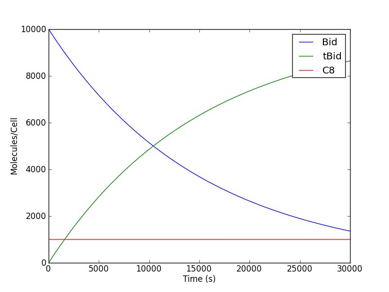
As you may recall we named some observables in the Observables section above. The variable yout contains an array of all the ODE outputs from the integrators along with the named observables (i.e. obsBid, obstBid, and obsC8) which can be called by their names. We can therefore plot this data to visualize our output. Using the commands imported from the PyLab module we can create a graph interactively. Enter the commands as shown below:

>>>pl.ion()
>>>pl.figure()
>>>pl.plot(t, yout['obsBid'], label="Bid")
>>>pl.plot(t, yout['obstBid'], label="tBid")
>>>pl.plot(t, yout['obsC8'], label="C8")
>>>pl.legend()
>>>pl.xlabel("Time (s)")
>>>pl.ylabel("Molecules/cell")
>>>pl.show()

You should now have a figure in your screen showing the number of Bid molecules decreaing from the initial amount decreasing over time, the number of tBid molecules increasing over time, and the number of free C8 molecules decrease to about half. For help with the above commands and to see more commands related to PyLab check the documentation [5]. Your figure should look something like the one below:

Congratulations! You have created your first model and run a simulation!

Visualization¶

It is useful to visualize the species and reactions that make a model. We have provided two methods to visualize species and reactions. We recommend using the tools in Kappa and BioNetGen for other visualization tools such as contact maps and stories.

The simplest way to visualize a model is to generate the graph file using the programs available from the command line. The files are located in the .../pysb/tools directory. The files to visualize reactions and species are render_reactions.py and render_species.py. These python scripts will generate .dot graph files that can be visualized using several tool such as OmniGraffle in OS X or GraphViz in all major platforms. For this tutorial we will use the GraphViz renderer. For this example will visualize the mymodel.py file that was created earlier. Issue the following command, replacing the comments inside square brackets``[]`` with the correct paths. We will first generate the .dot from the command line as follows:

[path-to-pysb]/pysb/tools/render_reactions.py [path-to-pysb-model-file]/mymodel.py > mymodel.dot

If your model can be properly visualized you should have gotten no errors and should now have a file called mymodel.dot. You can now use this file as an input for any visualization tool as described above. You can follow the same procedures with the render_species.py script to visualize the species generated by your models.

Advanced modeling¶

In this section we continue with the above tutorial and touch on some advanced techniques for modeling using compartments, the definition of higher order rules using functions, and model calibration using the PySB utilities. Although we provide the functions and utilities we have found useful for the community, we encourage users to customize the modeling tools to their needs and add/contribute to the PySB modeling community.

Higher-order rules¶

For this section we will show the power working in a programming environment by creating a simple function called “catalyze”. Catalysis happens quite often in models and it is one of the basic functions we have found useful in our model development. Rather than typing many lines such as:

Rule("association",  Enz(b=None) + Sub(b=None, S="i") <> Enz(b=1)%Sub(b=1,S="i"), kf, kr)
Rule("dissociation", Enz(b=1)%Sub(b=1,S="i") >> Enz(b=None) + Sub(b=None, S="a"), kc)

multiple times, we find it more powerful, transparent and easy to instantiate/edit a simple, one-line function call such as:

catalyze(Enz, Sub, "S", "i", "a", kf, kr, kc)

We find that the functional form captures what we mean to write: a chemical species (the substrate) undergoes catalytic activation (by the enzyme) with a given set of parameters. We will now describe how a function can be written in PySB to automate the scripting of simple concepts into a programmatic format. Examine the function below:

def catalyze(enz, sub, site, state1, state2, kf, kr, kc):   # (0) function call
    """2-step catalytic process"""                          # (1) reaction name
    r1_name = '%s_assoc_%s' % (enz.name, sub.name)          # (2) name of association reaction for rule
    r2_name = '%s_diss_%s' % (enz.name, sub.name)           # (3) name of dissociation reaction for rule
    E = enz(b=None)                                         # (4) define enzyme state in function
    S = sub({'b': None, site: state1})                      # (5) define substrate state in function
    ES = enz(b=1) % sub({'b': 1, site: state1})             # (6) define state of enzyme:substrate complex
    P = sub({'b': None, site: state2})                      # (7) define state of product
    Rule(r1_name, E + S <> ES, kf, kr)                      # (8) rule for enzyme + substrate association (bidirectional)
    Rule(r2_name, ES >> E + P, kc)                          # (9) rule for enzyme:substrate dissociation  (unidirectional)

As shown it takes about ten lines to write the catalyze function (shorter variants are certainly possible with more advanced Python statements). The skeleton of every function in Python

As shown, Monomers, Parameters, Species, and pretty much anything related to rules-based modeling are instantiated as objects in Python. One could write functions to interact with these objects and they could be instantiated and inherit methods from a class. The limits to programming biology with PySB are those enforced by the Python language itself. We can now go ahead and embed this into a model. Go back to your mymodel.py file and modify it to look something like this:

# import the pysb module and all its methods and functions
from pysb import *


def catalyze(enz, sub, site, state1, state2, kf, kr, kc):   # function call
    """2-step catalytic process"""                          # reaction name
    r1_name = '%s_assoc_%s' % (enz.name, sub.name)           # name of association reaction for rule
    r2_name = '%s_diss_%s' % (enz.name, sub.name)           # name of dissociation reaction for rule
    E = enz(b=None)                                         # define enzyme state in function
    S = sub({'b': None, site: state1})                      # define substrate state in function
    ES = enz(b=1) % sub({'b': 1, site: state1})             # define state of enzyme:substrate complex
    P = sub({'b': None, site: state2})                      # define state of product
    Rule(r1_name, E + S <> ES, kf, kr)                      # rule for enzyme + substrate association (bidirectional)
    Rule(r2_name, ES >> E + P, kc)                          # rule for enzyme:substrate dissociation  (unidirectional)
   
# instantiate a model
Model()

# declare monomers
Monomer('C8', ['b'])
Monomer('Bid', ['b', 'S'], {'S':['u', 't']})

# input the parameter values
Parameter('kf', 1.0e-07)
Parameter('kr', 1.0e-03)
Parameter('kc', 1.0)

# OLD RULES
# Rule('C8_Bid_bind', C8(b=None) + Bid(b=None, S=None) <> C8(b=1) % Bid(b=1, S=None), *[kf, kr]) 
# Rule('tBid_from_C8Bid', C8(b=1) % Bid(b=1, S='u') >> C8(b=None) + Bid(b=None, S='t'), kc)
#
# NEW RULES
# Catalysis
catalyze(C8, Bid, 'S', 'u', 't', kf, kr, kc)


# initial conditions
Parameter('C8_0', 1000)
Parameter('Bid_0', 10000)
Initial(C8(b=None), C8_0)
Initial(Bid(b=None, S='u'), Bid_0)

# Observables
Observable('obsC8', C8(b=None))
Observable('obsBid', Bid(b=None, S='u'))
Observable('obstBid', Bid(b=None, S='t'))

With this you should be able to execute your code and generate figures as described in the previous sections.

Using provided macros¶

For further reference we invite the users to explore the macros.py file in the .../pysb/ directory. Based on our experience with modeling signal transduction pathways we have identified a set of commonly-used constructs that can serve as building blocks for more complex models. In addition to some meta-macros useful for instantiating user macros, we provide a set of macros such as equilibrate. bind, catalyze, catalyze_one_step, catalyze_one_step_reversible, synthesize, degrade, assemble_pore_sequential, and pore_transport. In addition to these basic macros we also provide the higher-level macros bind_table and catalyze_table which we have found useful in instantiating the interactions between families of models.

In what follows we expand our previous model example of Caspase-8 by adding a few more species. The initiator caspase, as was described earlier, catalytically cleaves Bid to create truncated Bid (tBid) in this model. This tBid then catalytically activates Bax and Bak which eventually go on to form pores at the mitochondria leading to mitochondrial outer-membrane permeabilization (MOMP) and eventual cell death. To introduce the concept of higher-level macros we will show how the bind_table macro can be used to show how a family of inhibitors, namely Bcl-2, Bcl-xL, and Mcl-1 inhibits a family of proteins, namely Bid, Bax, and Bak.

In your favorite editor, go ahead and create a file (I will refer to it as ::file::mymodel_fxns). Many rules that dictate the interactions among species depend on a single binding site. We will begin by creating our model and declaring a generic binding site. We will also declare some functions, using the PySB macros and tailor them to our needs by specifying the binding site to be passed to the function. The first thing we do is import PySB and then import PySB macros. Then we declare our generic site and redefine the pysb.macros for our model as follows:

# import the pysb module and all its methods and functions
from pysb import *
from pysb.macros import *

# some functions to make life easy
site_name = 'b'
def catalyze_b(enz, sub, product, klist):
    """Alias for pysb.macros.catalyze with default binding site 'b'.
    """
    return catalyze(enz, site_name, sub, site_name, product, klist)
def bind_table_b(table):
    """Alias for pysb.macros.bind_table with default binding sites 'bf'.
    """
    return bind_table(table, site_name, site_name)

The first two lines just import the necessary modules from PySB. The catalyze_b` function, tailored for the model, takes four inputs but feeds six inputs to the pysb.macros.catalyze function, hence making the model more clean. Similarly the bind_table_b function takes only one entry, a list of lists, and feeds the entries needed to the pysb.macros.bind_table macro. Note that these entries could be contained in a header file to be hidden from the user at model time.

With this technical work out of the way we can now actually start our mdoel building. We will declare two sets of rates, the bid_rates that we will use for all the Bid interactions and the bcl2_rates which we will use for all the Bcl-2 interactions. Thesevalues could be specified individually as desired as desired but it is common practice in models to use generic values for the reaction rate parameters of a model and determine these in detail through some sort of model calibration. We will use these values for now for illustrative purposes.

The next entries for the rates, the model declaration, and the Monomers follow:

# Bid activation rates
bid_rates = [        1e-7, 1e-3, 1] #

# Bcl2 Inhibition Rates
bcl2_rates = [1.428571e-05, 1e-3] # 1.0e-6/v_mito

# instantiate a model
Model()

# declare monomers
Monomer('C8',    ['b'])
Monomer('Bid',   ['b', 'S'], {'S':['u', 't', 'm']})
Monomer('Bax',   ['b', 'S'], {'S':['i', 'a', 'm']})
Monomer('Bak',   ['b', 'S'], {'S':['i', 'a']})
Monomer('BclxL', ['b', 'S'], {'S':['c', 'm']})
Monomer('Bcl2', ['b'])
Monomer('Mcl1', ['b'])

As shown, the generic rates are declared followed by the declaration of the monomers. We have the C8 and Bid monomers as we did in the initial part of the tutorial, the MOMP effectors Bid, Bax, Bak, and the MOMP inhibitors Bcl-xL, Bcl-2, and Mcl-1. The Bid, Bax, and BclxL monomers, in addition to the active and inactive terms also have a 'm' term indicating that they can be in a membrane, which in this case we indicate as a state. We will have a translocation to the membrane as part of the reactions.

We can now begin to write some checmical procedures. The first procedure is the catalytic activation of Bid by C8. This is followed by the catalytic activation of Bax and Bak.

# Activate Bid
catalyze_b(C8, Bid(S='u'), Bid(S='t'), [KF, KR, KC])

# Activate Bax/Bak
catalyze_b(Bid(S='m'), Bax(S='i'), Bax(S='m'), bid_rates)
catalyze_b(Bid(S='m'), Bak(S='i'), Bak(S='a'), bid_rates)

As shown, we simply state the soecies that acts as an enzyme as the first function argument, the species that acts as the reactant with the enzyme as the second argument (along with any state specifications) and finally the product species. The bid_rates argument is the list of rates that we declared earlier.

You may have noticed a problem with the previous statements. The Bid species undergoes a transformation from state S='u' to S='t' but the activation of Bax and Bak happens only when Bid is in state S='m' to imply that these events only happen at the membrane. In order to transport Bid from the 't' state to the 'm' state we need a transporf function. We achieve this by using the equilibrate macro in PySB between these states. In addition we use this same macro for the transport of the Bax species and the BclxL species as shown below.

# Bid, Bax, BclxL "transport" to the membrane
equilibrate(Bid(b=None, S='t'),   Bid(b=None, S='m'), [1e-1, 1e-3])
equilibrate(Bax(b=None, S='m'),   Bax(b=None, S='a'), [1e-1, 1e-3])
equilibrate(BclxL(b=None, S='c'), BclxL(b=None, S='m'), [1e-1, 1e-3])

According to published experimental data, the Bcl-2 family of inhibitors can inhibit the initiator Bid and the effector Bax and Bak. These family has complex interactions with all these proteins. Given that we have three inhibitors, and three molecules to be inhibited, this indicates nine interactions that need to be specified. This would involve writing nine reversible reactions in a rules language or at least eighteen reactions for each direction if we were writing the ODEs. Given that we are simply stating that these species bind to inhibit interactions, we can take advantage of two things. In the first case we have already seen that there is a bind macro specified in PySB. We can further functionalize this into a higher level macro, naemly the bind_table macro, which takes a table of interactions as an argument and generates the rules based on these simple interactions. We specify the bind table for the inhibitors (top row) and the inhibited molecules (left column) as follows.

bind_table_b([[                  Bcl2,  BclxL(S='m'),       Mcl1],
              [Bid(S='m'), bcl2_rates,  bcl2_rates,   bcl2_rates],
              [Bax(S='a'), bcl2_rates,  bcl2_rates,         None],
              [Bak(S='a'),       None,  bcl2_rates,   bcl2_rates]])

As shown the inhibitors interact by giving the rates of interactions or the “None” Python keyword to indicate no interaction. The only thing left to run this simple model is to declare some initial conditions and some observables. We declare the following:

# initial conditions
Parameter('C8_0',    1e4)
Parameter('Bid_0',   1e4)
Parameter('Bax_0',  .8e5)
Parameter('Bak_0',  .2e5)
Parameter('BclxL_0', 1e3)
Parameter('Bcl2_0',  1e3)
Parameter('Mcl1_0',  1e3)

Initial(C8(b=None), C8_0)
Initial(Bid(b=None, S='u'), Bid_0)
Initial(Bax(b=None, S='i'), Bax_0)
Initial(Bak(b=None, S='i'), Bak_0)
Initial(BclxL(b=None, S='c'), BclxL_0)
Initial(Bcl2(b=None), Bcl2_0)
Initial(Mcl1(b=None), Mcl1_0)

# Observables
Observable('obstBid', Bid(b=None, S='m'))
Observable('obsBax', Bax(b=None, S='a'))
Observable('obsBak', Bax(b=None, S='a'))
Observable('obsBaxBclxL', Bax(b=1, S='a')%BclxL(b=1, S='m'))

By now you should have a file with all the components that looks something like this:

# import the pysb module and all its methods and functions
from pysb import *
from pysb.macros import *

# some functions to make life easy
site_name = 'b'
def catalyze_b(enz, sub, product, klist):
    """Alias for pysb.macros.catalyze with default binding site 'b'.
    """
    return catalyze(enz, site_name, sub, site_name, product, klist)

def bind_table_b(table):
    """Alias for pysb.macros.bind_table with default binding sites 'bf'.
    """
    return bind_table(table, site_name, site_name)

# Default forward, reverse, and catalytic rates
KF = 1e-6
KR = 1e-3
KC = 1

# Bid activation rates
bid_rates = [        1e-7, 1e-3, 1] #

# Bcl2 Inhibition Rates
bcl2_rates = [1.428571e-05, 1e-3] # 1.0e-6/v_mito

# instantiate a model
Model()

# declare monomers
Monomer('C8',    ['b'])
Monomer('Bid',   ['b', 'S'], {'S':['u', 't', 'm']})
Monomer('Bax',   ['b', 'S'], {'S':['i', 'a', 'm']})
Monomer('Bak',   ['b', 'S'], {'S':['i', 'a']})
Monomer('BclxL', ['b', 'S'], {'S':['c', 'm']})
Monomer('Bcl2', ['b'])
Monomer('Mcl1', ['b'])

# Activate Bid
catalyze_b(C8, Bid(S='u'), Bid(S='t'), [KF, KR, KC])

# Activate Bax/Bak
catalyze_b(Bid(S='m'), Bax(S='i'), Bax(S='m'), bid_rates)
catalyze_b(Bid(S='m'), Bak(S='i'), Bak(S='a'), bid_rates)

# Bid, Bax, BclxL "transport" to the membrane
equilibrate(Bid(b=None, S='t'),   Bid(b=None, S='m'), [1e-1, 1e-3])
equilibrate(Bax(b=None, S='m'),   Bax(b=None, S='a'), [1e-1, 1e-3])
equilibrate(BclxL(b=None, S='c'), BclxL(b=None, S='m'), [1e-1, 1e-3])


bind_table_b([[                  Bcl2,  BclxL(S='m'),       Mcl1],
              [Bid(S='m'), bcl2_rates,  bcl2_rates,   bcl2_rates],
              [Bax(S='a'), bcl2_rates,  bcl2_rates,         None],
              [Bak(S='a'),       None,  bcl2_rates,   bcl2_rates]])

# initial conditions
Parameter('C8_0',    1e4)
Parameter('Bid_0',   1e4)
Parameter('Bax_0',  .8e5)
Parameter('Bak_0',  .2e5)
Parameter('BclxL_0', 1e3)
Parameter('Bcl2_0',  1e3)
Parameter('Mcl1_0',  1e3)

Initial(C8(b=None), C8_0)
Initial(Bid(b=None, S='u'), Bid_0)
Initial(Bax(b=None, S='i'), Bax_0)
Initial(Bak(b=None, S='i'), Bak_0)
Initial(BclxL(b=None, S='c'), BclxL_0)
Initial(Bcl2(b=None), Bcl2_0)
Initial(Mcl1(b=None), Mcl1_0)

# Observables
Observable('obstBid', Bid(b=None, S='m'))
Observable('obsBax', Bax(b=None, S='a'))
Observable('obsBak', Bax(b=None, S='a'))
Observable('obsBaxBclxL', Bax(b=1, S='a')%BclxL(b=1, S='m'))

With this you should be able to run the simulations and generate figures as described in the basic tutorial sections.

Compartments¶

We will continue building on your mymodel_fxns.py file and add one more species and a compartment. In extrinsic apoptosis, once tBid is activated it translocates to the outer mitochondrial membrane where it interacts with the protein Bak (residing in the membrane).

Model calibration¶

COMING SOON: ANNEAL

Modules¶

Footnotes

[1]	Technically speaking it’s a constructor, not just any old function.

[2]	Python allows users to write PySB code to a file. This file can be later used as an executable script or from an interactive instance. Such files are called modules and can be imported into a Python instance. See Python modules for details.

[3]	The astute Python programmer will recognize this as the `repr` of the monomer object, using keyword arguments in the constructor call.

[4]	SciPy: http://www.scipy.org

[5]	(1, 2) PyLab: http://www.scipy.org/PyLab

Tutorial¶

Modeling with PySB¶

The Empty Model¶

Monomers¶

Parameters¶

Rules¶

Initial conditions¶

Observables¶

Simulation and analysis¶

Visualization¶

Advanced modeling¶

Higher-order rules¶

Using provided macros¶

Compartments¶

Model calibration¶

Modules¶

Project Versions

Table Of Contents

Previous topic

Next topic

This Page

Navigation

Tutorial¶

Modeling with PySB¶

The Empty Model¶

Monomers¶

Parameters¶

Rules¶

Initial conditions¶

Observables¶

Simulation and analysis¶

Visualization¶

Advanced modeling¶

Higher-order rules¶

Using provided macros¶

Compartments¶

Model calibration¶

Modules¶

Project Versions

RTD Search

Table Of Contents

Previous topic

Next topic

This Page

Quick search

Navigation